Parent Faults

This notebook demonstrates parent-fault-level view classes. Topics covered:

1. Creating a ParentFault facade

2. ParentFaultData — subsection attributes and geometry (oriented surface trace)

3. Constructing parent fault dimension tables from ds.subsections

4. ParentFaultRuptures — participating ruptures and cumulative MFDs

5. Direct instantiation of ParentFaultData and ParentFaultRuptures

import matplotlib.pyplot as plt
import pandas as pd

from parserf import (
    FaultModel,
    FaultModelDataset,
    ParentFault,
    ParentFaultData,
    ParentFaultRuptures,
)

ds = FaultModelDataset(FaultModel.NSHMP_2023)

1. ParentFault Facade

ParentFault validates the name and exposes .data and .ruptures.

flt = ParentFault(ds, name="Compton")
print(flt)

ParentFault(fault_model=NSHMP_2023, name='Compton', parent_id=43)

2. ParentFaultData

print("Name:       ", flt.data.name)
print("Parent ID:  ", flt.data.parent_id)
print("Fault Model:", flt.data.fault_model.name)

Name:        Compton
Parent ID:   43
Fault Model: NSHMP_2023

Child subsections

# Get the subsections for this parent fault
subs = flt.data.subsections
print(f"{len(subs)} subsections")
subs

5 subsections

	name	dip	dip_direction	upper_depth_km	lower_depth_km	aseismicity	length_km	width_km	area_km2	geometry
index
809	Compton (0)	20.0	34.0	5.2	15.6	0.1	12.978331	30.407566	394.639455	LINESTRING (-118.06065 33.68127, -118.13114 33...
810	Compton (1)	20.0	34.0	5.2	15.6	0.1	12.983062	30.407566	394.783297	LINESTRING (-118.1787 33.74269, -118.22804 33....
811	Compton (2)	20.0	34.0	5.2	15.6	0.1	12.985653	30.407566	394.862090	LINESTRING (-118.30314 33.79592, -118.31471 33...
812	Compton (3)	20.0	34.0	5.2	15.6	0.1	12.979565	30.407566	394.676979	LINESTRING (-118.43104 33.84393, -118.43655 33...
813	Compton (4)	20.0	34.0	5.2	15.6	0.1	12.954084	30.407566	393.902164	LINESTRING (-118.55061 33.90376, -118.5863 33....

# Statistics for the subsections in the parent fault
subs[["dip", "upper_depth_km", "lower_depth_km", "length_km", "width_km", "area_km2"]].describe()

	dip	upper_depth_km	lower_depth_km	length_km	width_km	area_km2
count	5.0	5.0	5.0	5.000000	5.000000	5.000000
mean	20.0	5.2	15.6	12.976139	30.407566	394.572797
std	0.0	0.0	0.0	0.012663	0.000000	0.385048
min	20.0	5.2	15.6	12.954084	30.407566	393.902164
25%	20.0	5.2	15.6	12.978331	30.407566	394.639455
50%	20.0	5.2	15.6	12.979565	30.407566	394.676979
75%	20.0	5.2	15.6	12.983062	30.407566	394.783297
max	20.0	5.2	15.6	12.985653	30.407566	394.862090

Per-subsection scalars (dip, dip_direction, …) are not pre-aggregated at the parent level — ParentFaultData exposes the raw data.subsections and leaves aggregation to you. For example, an area-weighted dip and dip direction (reused in the plot titles further down):

# Aggregate per-subsection scalars yourself, e.g. area-weighted dip / dip direction:
weights = subs["area_km2"]
dip = (subs["dip"] * weights).sum() / weights.sum()
dip_direction = (subs["dip_direction"] * weights).sum() / weights.sum()
print(f"Area-weighted dip:           {dip:.1f}°")
print(f"Area-weighted dip direction: {dip_direction:.1f}°")

Area-weighted dip:           20.0°
Area-weighted dip direction: 34.0°

Surface trace (data.geometry)

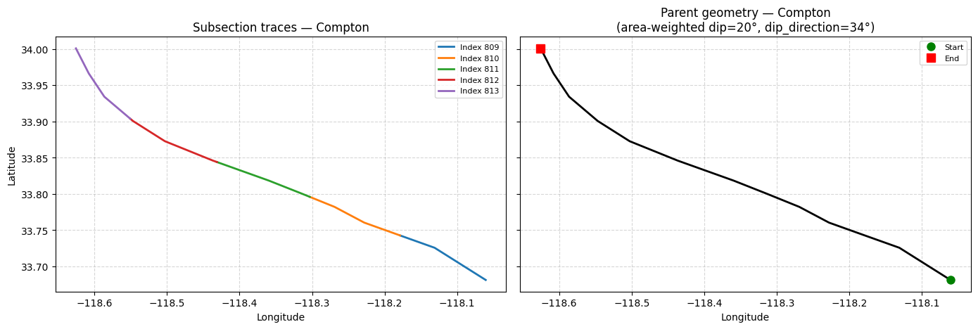
Individual subsection traces vs. the merged and oriented parent geometry (right-hand rule: dip direction to the right as you walk the coordinates).

fig, (ax1, ax2) = plt.subplots(1, 2, figsize=(14, 6), sharey=True)

# Left: access the individual subsection traces
for idx, row in subs.iterrows():
    xs, ys = row["geometry"].xy
    # This is a shapely LineString object, so we can get the x and y coordinates directly
    ax1.plot(xs, ys, linewidth=2, label=f"Index {idx}")
ax1.set_xlabel("Longitude")
ax1.set_ylabel("Latitude")
ax1.set_title(f"Subsection traces — {flt.data.name}")
ax1.legend(fontsize=8)
ax1.set_aspect("equal")
ax1.grid(True, linestyle="--", alpha=0.5)

# Right: Parent geometry is readily available and oriented with dip on the right
trace = flt.data.geometry
lons, lats = trace.xy
ax2.plot(lons, lats, linewidth=2, color="black")
ax2.plot(lons[0], lats[0], "o", color="green", markersize=8, label="Start")
ax2.plot(lons[-1], lats[-1], "s", color="red", markersize=8, label="End")
ax2.set_xlabel("Longitude")
ax2.set_title(
    f"Parent geometry — {flt.data.name}\n"
    f"(area-weighted dip={dip:.0f}°, dip_direction={dip_direction:.0f}°)"
)
ax2.legend(fontsize=8)
ax2.set_aspect("equal")
ax2.grid(True, linestyle="--", alpha=0.5)

plt.tight_layout()
plt.show()

Footprint (data.geometry_3d)

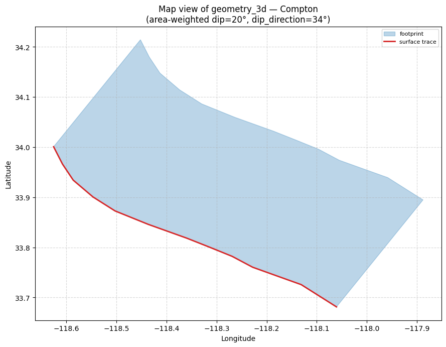
The 3D counterpart to geometry: the child subsection surfaces are stitched into a single PolygonZ. This provides the parent fault footprint in map view.

footprint = flt.data.geometry_3d
fx, fy = footprint.exterior.xy
tx, ty = flt.data.geometry.xy

fig, ax = plt.subplots(figsize=(9, 7))
ax.fill(fx, fy, alpha=0.3, color="tab:blue", label="footprint")
ax.plot(tx, ty, color="tab:red", linewidth=2, label="surface trace")
ax.set_xlabel("Longitude")
ax.set_ylabel("Latitude")
ax.set_title(
    f"Map view of geometry_3d — {flt.data.name}\n"
    f"(area-weighted dip={dip:.0f}°, dip_direction={dip_direction:.0f}°)"
)
ax.legend(fontsize=8)
ax.set_aspect("equal")
ax.grid(True, linestyle="--", alpha=0.5)
plt.tight_layout()
plt.show()

3. Constructing per-parent data summaries

Earthquake rupture forecasts (ERFs) are built at the subsection level. Parent-level summaries are easy to build from ds.subsections, so consumers can choose the aggregation that matches their workflow.

parent_dimensions = (
    ds.subsections.assign(length_meters=ds.subsections["length_km"] * 1000.0)
    .groupby("parent_id")
    .agg(
        parent_name=("parent_name", "first"),
        length_meters=("length_meters", "sum"),
        dip_degrees_min=("dip", "min"),
        dip_degrees_max=("dip", "max"),
        dip_degrees_mean=("dip", "mean"),
        upper_depth_km_min=("upper_depth_km", "min"),
        upper_depth_km_max=("upper_depth_km", "max"),
        upper_depth_km_mean=("upper_depth_km", "mean"),
        lower_depth_km_min=("lower_depth_km", "min"),
        lower_depth_km_max=("lower_depth_km", "max"),
        lower_depth_km_mean=("lower_depth_km", "mean"),
    )
    .reset_index()
)

parent_dimensions.head()

	parent_id	parent_name	length_meters	dip_degrees_min	dip_degrees_max	dip_degrees_mean	upper_depth_km_min	upper_depth_km_max	upper_depth_km_mean	lower_depth_km_min	lower_depth_km_max	lower_depth_km_mean
0	1	Airport Lake	47122.932031	50.0	50.0	50.0	0.0	0.0	0.0	13.0	13.0	13.0
1	2	Almanor	34542.069300	90.0	90.0	90.0	0.0	0.0	0.0	10.0	10.0	10.0
2	3	Anacapa - Dume	64887.004711	45.0	45.0	45.0	0.0	0.0	0.0	15.5	15.5	15.5
3	5	Anaheim	15721.571346	71.0	71.0	71.0	3.8	3.8	3.8	14.2	14.2	14.2
4	6	Ash Hill	49118.249711	90.0	90.0	90.0	0.0	0.0	0.0	13.0	13.0	13.0

4. ParentFaultRuptures

participating_ruptures

GeoDataFrame of all ruptures involving any child subsection of this parent fault. The contributions column lists (parent_id, area_pct) tuples for every parent each rupture touches, so you can see the relative contribution of this parent and other parents for every rupture.

rups = flt.ruptures.participating_ruptures
print(f"{len(rups)} ruptures")
print("Columns:", list(rups.columns))
rups.head()

7230 ruptures
Columns: ['m', 'rate', 'depth', 'dip', 'width', 'rake', 'geometry', 'length_km', 'area_km2', 'contributions']

	m	rate	depth	dip	width	rake	geometry	length_km	area_km2	contributions
1956	7.15	1.669645e-09	3.241	45.1	21.252	71.0	MULTILINESTRING ((-118.552 34.0202, -118.64926...	49.174780	1088.344469	[(3, 43.56092257573472), (43, 36.1927840965310...
1957	7.36	5.858259e-10	3.296	38.5	22.825	71.0	MULTILINESTRING ((-118.552 34.0202, -118.64926...	71.108453	1711.583027	[(3, 27.69908814193388), (43, 23.0139091992105...
1958	7.41	5.821115e-11	3.870	37.2	21.902	73.0	MULTILINESTRING ((-118.552 34.0202, -118.64926...	82.976216	1860.481866	[(3, 25.482263500431234), (43, 21.172050696551...
1960	7.45	1.333749e-11	4.359	36.0	21.115	75.0	MULTILINESTRING ((-118.552 34.0202, -118.64926...	94.840401	2009.335812	[(3, 23.594507625457194), (43, 19.603600425759...
1961	7.42	3.768216e-09	3.395	39.7	21.869	72.0	MULTILINESTRING ((-118.552 34.0202, -118.64926...	84.560123	1922.301928	[(3, 24.662769386835574), (43, 20.491170408257...

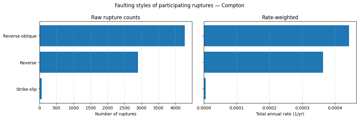
Working with rakes. parserf exposes each rupture’s raw rake (which is provided by the ERF) but does not classify styles of faulting. Here’s an example of how you can do that: classify each rupture’s rake into a style, then compare a raw rupture count against a rate-weighted tally. The two can differ significantly in some cases; the counts reflect how the inversion enumerated ruptures, while rate-weighting generallly will better reflect the underlying forecast itself.

# Classify each rupture's rake into a style of faulting — your convention, your choice
def classify_rake(rake):
    rake = ((rake + 180) % 360) - 180  # normalize to [-180, 180)
    ranges = [
        ((-20, 20), "Strike-slip"),
        ((20, 70), "Reverse oblique"),
        ((70, 110), "Reverse"),
        ((110, 160), "Reverse oblique"),
        ((160, 180), "Strike-slip"),
        ((-180, -160), "Strike-slip"),
        ((-160, -110), "Normal oblique"),
        ((-110, -70), "Normal"),
        ((-70, -20), "Normal oblique"),
    ]
    for (low, high), label in ranges:
        if low <= rake < high:
            return label


styles = rups["rake"].apply(classify_rake)
counts = styles.value_counts()  # raw: one tally per rupture
rates = rups.groupby(styles)["rate"].sum()  # rate-weighted: sum of annual rates

order = counts.index  # same category order on both panels
fig, (ax1, ax2) = plt.subplots(1, 2, figsize=(12, 4), sharey=True)

ax1.barh(order, counts.loc[order])
ax1.set_xlabel("Number of ruptures")
ax1.set_title("Raw rupture counts")
ax1.invert_yaxis()
ax1.grid(axis="x", linestyle="--", alpha=0.5)

ax2.barh(order, rates.reindex(order, fill_value=0.0))
ax2.set_xlabel("Total annual rate (1/yr)")
ax2.set_title("Rate-weighted")
ax2.grid(axis="x", linestyle="--", alpha=0.5)

fig.suptitle(f"Faulting styles of participating ruptures — {flt.data.name}")
plt.tight_layout()
plt.show()

Each rupture’s contributions lists (parent_id, area_pct) for every parent it touches. To attribute a rupture’s rate to individual faults:

• Explode contributions to one row per (rupture, parent) and split the tuples into parent_id / area_pct

• Keep this parent’s rows and scale each rupture’s rate by its area share (rate × area_pct / 100)

# Each rupture's `contributions` lists (parent_id, area_pct) for every parent it touches.
# Explode that column into one row per (rupture, parent), then split the tuples into columns:
exploded = rups.explode("contributions")
exploded[["parent_id", "area_pct"]] = pd.DataFrame(
    exploded["contributions"].tolist(), index=exploded.index
)

# Keep this parent's rows and attribute each rupture's rate to it by area:
this_parent = exploded[exploded["parent_id"] == flt.data.parent_id].copy()
this_parent["attributed_rate"] = (
    this_parent["rate"] * this_parent["area_pct"] / 100.0
)  # full rate × this parent's area share

print(f"{len(this_parent)} (rupture, {flt.data.name}) contributions")
this_parent[["m", "rate", "area_pct", "attributed_rate"]].head()

7230 (rupture, Compton) contributions

	m	rate	area_pct	attributed_rate
1956	7.15	1.669645e-09	36.192784	6.042910e-10
1957	7.36	5.858259e-10	23.013909	1.348214e-10
1958	7.41	5.821115e-11	21.172051	1.232449e-11
1960	7.45	1.333749e-11	19.603600	2.614629e-12
1961	7.42	3.768216e-09	20.491170	7.721515e-10

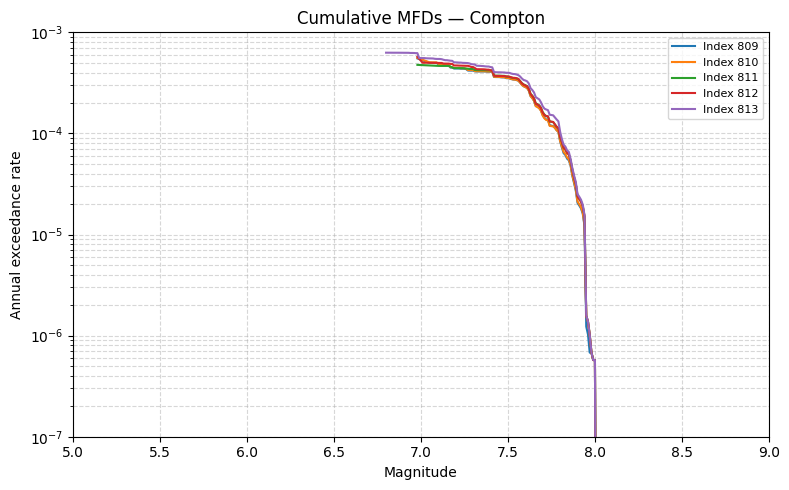
cumulative_mfds

Cumulative magnitude frequency distributions for each child subsection.

mfds = flt.ruptures.cumulative_mfds
subsection_indices = sorted(int(i) for i in mfds["index"].unique())
print(f"Total rows: {len(mfds)}")
print(f"Subsection indices: {subsection_indices}")
mfds.head()

Total rows: 495
Subsection indices: [809, 810, 811, 812, 813]

	index	magnitude	cumulative_rate
0	809	6.98	0.000552
1	809	7.05	0.000499
2	809	7.07	0.000499
3	809	7.09	0.000499
4	809	7.11	0.000469

# Plot the cumulative MFDs for each subsection in the parent fault
fig, ax = plt.subplots(figsize=(8, 5))
for idx, group in mfds.groupby("index"):
    ax.semilogy(group["magnitude"], group["cumulative_rate"], linewidth=1.5, label=f"Index {idx}")
ax.set_xlabel("Magnitude")
ax.set_ylabel("Annual exceedance rate")
ax.set_title(f"Cumulative MFDs \u2014 {flt.data.name}")
ax.set(xlim=(5, 9), ylim=(1e-7, 1e-3))
ax.legend(fontsize=8)
ax.grid(True, which="both", linestyle="--", alpha=0.5)
plt.tight_layout()
plt.show()

5. Direct Instantiation

ParentFaultData and ParentFaultRuptures can be used standalone. They take parent_id (an integer) rather than name.

pid = ds.get_parent_fault_id(name="Compton")

data = ParentFaultData(ds, parent_id=pid)
print("Name:", data.name)
print("Subsections:", len(data.subsections))

Name: Compton
Subsections: 5

ruptures = ParentFaultRuptures(ds, parent_id=pid)
print("Cumulative MFD rows:", len(ruptures.cumulative_mfds))

Cumulative MFD rows: 495