Fault Subsections

This notebook demonstrates subsection-level view classes. Topics covered:

1. Creating a FaultSubsection facade

2. FaultSubsectionData — subsection attributes

3. FaultSubsectionRuptures — rupture participation and cumulative MFD

4. Direct instantiation of FaultSubsectionData and FaultSubsectionRuptures

import matplotlib.pyplot as plt
import numpy as np

from parserf import (
    FaultModel,
    FaultModelDataset,
    FaultSubsection,
    FaultSubsectionData,
    FaultSubsectionRuptures,
    get_nearest_subsection_index,
)

# Coordinate in southern California (nearest parent fault: Compton)
ds = FaultModelDataset(FaultModel.NSHMP_2023)
idx = get_nearest_subsection_index(ds, lat=33.85, lon=-118.40)
print("Nearest subsection index:", idx)

Nearest subsection index: 811

1. FaultSubsection Facade

FaultSubsection validates the index and exposes .data and .ruptures.

sub = FaultSubsection(ds, index=idx)
print(sub)

FaultSubsection(fault_model=NSHMP_2023, index=811, name='Compton (2)')

2. FaultSubsectionData

Properties for a single subsection’s attributes.

print("Index:       ", sub.data.index)
print("Name:        ", sub.data.name)
print("Parent ID:   ", sub.data.parent_id)
print("Parent Name: ", sub.data.parent_name)

Index:        811
Name:         Compton (2)
Parent ID:    43
Parent Name:  Compton

print("Geometry:    ", sub.data.geometry)
print("Length (km): ", round(sub.data.length_km, 3))
print("Width (km):  ", round(sub.data.width_km, 3))
print("Area (km\u00b2):  ", round(sub.data.area_km2, 3))

Geometry:     LINESTRING (-118.30314 33.79592, -118.31471 33.8006, -118.35945 33.8183, -118.43104 33.84393)
Length (km):  12.986
Width (km):   30.408
Area (km²):   394.862

print("Upper depth (km):  ", sub.data.upper_depth_km)
print("Lower depth (km):  ", sub.data.lower_depth_km)
print("Dip (degrees):     ", sub.data.dip)
print("Dip direction:     ", sub.data.dip_direction)
print("Aseismicity:       ", sub.data.aseismicity)

Upper depth (km):   5.2
Lower depth (km):   15.6
Dip (degrees):      20.0
Dip direction:      34.0
Aseismicity:        0.1

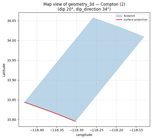
geometry_3d (dipping surface, map view)

geometry_3d is the dipping fault surface as a Shapely PolygonZ in (lon, lat, depth_km), built by hanging the top trace (surface projection or surface trace) down-dip to the lower seismogenic depth.

# Get the footprint with Shapely's `.exterior.xy`
footprint = sub.data.geometry_3d
fx, fy = footprint.exterior.xy
tx, ty = sub.data.geometry.xy

fig, ax = plt.subplots(figsize=(7, 6))
ax.fill(fx, fy, alpha=0.3, color="tab:blue", label="footprint")
ax.plot(tx, ty, color="tab:red", linewidth=2, label="surface projection")
ax.set_xlabel("Longitude")
ax.set_ylabel("Latitude")
ax.set_title(
    f"Map view of geometry_3d — {sub.data.name}\n"
    f"(dip {sub.data.dip:.0f}°, dip_direction {sub.data.dip_direction:.0f}°)"
)
ax.legend(fontsize=8)
ax.set_aspect("equal")
ax.grid(True, linestyle="--", alpha=0.5)
plt.tight_layout()
plt.show()

3. FaultSubsectionRuptures

Rupture participation data for a single subsection.

participating_ruptures

GeoDataFrame of all rupture scenarios involving this subsection, enriched with merged geometry and total length/area. There is one row per rupture.

What is the contributions column? A rupture can span subsections from several parent faults, so each rupture row carries a contributions list of (parent_id, area_pct) tuples — each parent’s share, by area, of the rupture (percentages sum to 100). That lets you attribute a rupture’s rate to individual faults via rate * area_pct / 100. Explode the column to get one row per (rupture, parent).

rups = sub.ruptures.participating_ruptures
print(f"{len(rups)} ruptures")
print("Columns:", list(rups.columns))
rups.head()

5190 ruptures
Columns: ['m', 'rate', 'depth', 'dip', 'width', 'rake', 'geometry', 'length_km', 'area_km2', 'contributions']

	m	rate	depth	dip	width	rake	geometry	length_km	area_km2	contributions
1975	7.66	4.321805e-15	4.682	34.3	23.885	71.0	MULTILINESTRING ((-118.552 34.0202, -118.64926...	127.177358	3176.545047	[(3, 14.924796731279569), (43, 62.107225134700...
2039	7.33	2.931294e-09	4.900	27.1	25.184	61.0	MULTILINESTRING ((-118.552 34.0202, -118.64926...	60.547321	1657.534124	[(3, 28.6023005259089), (43, 71.3976994740911)]
2040	7.43	1.801956e-09	5.158	25.8	25.604	62.0	MULTILINESTRING ((-118.552 34.0202, -118.64926...	73.530383	2052.317420	[(3, 23.100368715752083), (43, 76.899631284247...
2041	7.52	1.494799e-09	5.332	24.8	25.888	63.0	MULTILINESTRING ((-118.552 34.0202, -118.64926...	86.508714	2446.956875	[(3, 19.374795532753385), (43, 80.625204467246...
2042	7.55	1.325219e-09	5.310	26.9	25.168	65.0	MULTILINESTRING ((-118.552 34.0202, -118.64926...	96.988993	2562.232141	[(3, 18.50312014207105), (5, 4.499017237156169...

# Examine the parent fault contribution for one rupture via its `contributions` list.
last_rup_idx = rups.index[-1]
row = rups.loc[last_rup_idx]
print("Length (km):            ", round(row["length_km"], 2))
print("Area (km²):             ", round(row["area_km2"], 2))
print("Geometry type:          ", row["geometry"].geom_type)
print("Parent area breakdown:")
for pid, area_pct in row["contributions"]:
    pname = ds.subsections.loc[ds.subsections["parent_id"] == pid, "parent_name"].iloc[0]
    print(f"  {pname} (id={pid}): {area_pct:.1f}%")

Length (km):             127.77
Area (km²):              3500.29
Geometry type:           MultiLineString
Parent area breakdown:
  Compton (id=43): 56.4%
  Yorba Linda (id=303): 6.7%
  Santa Monica (id=262): 7.7%
  Santa Monica Bay (id=261): 22.2%
  Peralta Hills (id=206): 7.1%

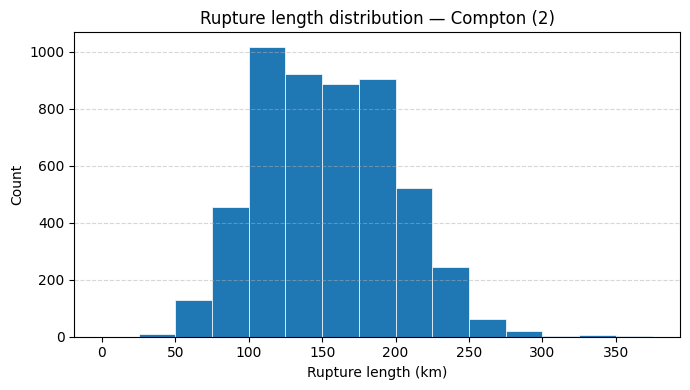
# Distribution of rupture lengths for this subsection
bin_width = 25
lengths = rups["length_km"]
bins = np.arange(0, lengths.max() + bin_width, bin_width)

fig, ax = plt.subplots(figsize=(7, 4))
ax.hist(lengths, bins=bins, edgecolor="white", linewidth=0.5)
ax.set_xlabel("Rupture length (km)")
ax.set_ylabel("Count")
ax.set_title(f"Rupture length distribution — {sub.data.name}")
ax.grid(axis="y", linestyle="--", alpha=0.5)
plt.tight_layout()
plt.show()

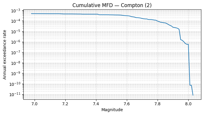
cumulative_mfd

Cumulative magnitude frequency distribution (exceedance rates).

mfd = sub.ruptures.cumulative_mfd
mfd

	magnitude	cumulative_rate
0	6.98	4.766730e-04
1	7.10	4.656969e-04
2	7.16	4.655489e-04
3	7.19	4.423972e-04
4	7.20	4.423908e-04
...	...	...
83	7.99	5.733441e-07
84	8.00	5.733367e-07
85	8.01	7.313346e-11
86	8.02	7.035943e-11
87	8.03	8.098438e-12

88 rows × 2 columns

# Cumulative MFD for this subsection
fig, ax = plt.subplots(figsize=(7, 4))
ax.semilogy(mfd["magnitude"], mfd["cumulative_rate"], linewidth=1.5)
ax.set_xlabel("Magnitude")
ax.set_ylabel("Annual exceedance rate")
ax.set_title(f"Cumulative MFD \u2014 {sub.data.name}")
ax.grid(True, which="both", linestyle="--", alpha=0.5)
plt.tight_layout()
plt.show()

4. Direct Instantiation

FaultSubsectionData and FaultSubsectionRuptures can be used standalone without going through the FaultSubsection facade.

data = FaultSubsectionData(ds, index=idx)
print("Name:", data.name)
print("Length (km):", round(data.length_km, 3))

Name: Compton (2)
Length (km): 12.986

ruptures = FaultSubsectionRuptures(ds, index=idx)
print("Participating ruptures:", len(ruptures.participating_ruptures))

Participating ruptures: 5190