Queries
This notebook demonstrates query functions and batch selection classes. Topics covered:
Lookups and spatial queries —
get_parent_fault_id,get_nearest_subsection_index,get_subsections_list,get_parents_list,get_ruptures_nearParentSelection— batch access to parent fault summaries, subsection attributes, and enriched rupturesGridSelection— background gridded seismicity within a search radius
import matplotlib.pyplot as plt
import numpy as np
import pandas as pd

from parserf import (
    FaultModel,
    FaultModelDataset,
    GridSelection,
    ParentSelection,
    get_nearest_subsection_index,
    get_parents_list,
    get_ruptures_near,
    get_subsections_list,
)
ds = FaultModelDataset(FaultModel.NSHMP_2023)
1. Lookups and Spatial Queries
get_parent_fault_id
Resolve a parent fault name to its integer ID.
pid = ds.get_parent_fault_id(name="Little Lake")
print("Parent ID for 'Little Lake':", pid)
Parent ID for 'Little Lake': 145
get_nearest_subsection_index
Find the closest subsection to a geographic coordinate.
# Coordinate near Ridgecrest, CA
idx = get_nearest_subsection_index(ds, lat=35.77, lon=-117.60)
print("Nearest subsection index:", idx)
print("Name:", ds.subsections.loc[idx, "name"])
Nearest subsection index: 3276
Name: Paxton Ranch (4)
get_subsections_list
Find all subsection indices within a search radius, sorted by distance.
nearby_subs = get_subsections_list(ds, lat=35.77, lon=-117.60, dist_km=50.0)
print(f"{len(nearby_subs)} subsections within 50 km")
print("First 10:", nearby_subs[:10])
79 subsections within 50 km
First 10: [3276, 3275, 3277, 16, 17, 3274, 18, 3758, 3759, 2447]
get_parents_list
Find all parent fault IDs within a search radius, sorted by nearest child subsection.
parent_ids = get_parents_list(ds, lat=35.77, lon=-117.60, dist_km=50.0)
print(f"{len(parent_ids)} parent faults within 50 km")

# Look up names for the parent IDs
pid_to_name = ds.parent_ids.set_index("parent_id")["parent_name"]
for pid in parent_ids:
    print(f"  {pid}: {pid_to_name[pid]}")
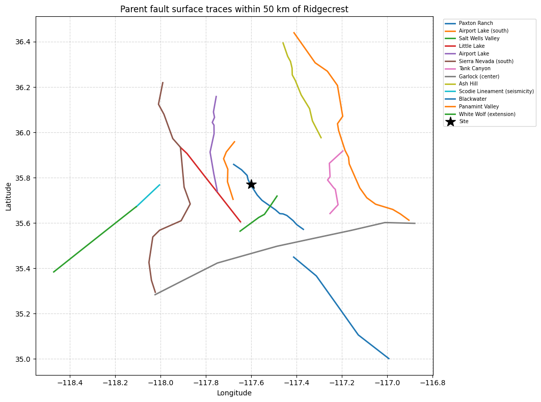
13 parent faults within 50 km
  331: Paxton Ranch
  310: Airport Lake (south)
  338: Salt Wells Valley
  145: Little Lake
  1: Airport Lake
  278: Sierra Nevada (south)
  287: Tank Canyon
  881: Garlock (center)
  6: Ash Hill
  272: Scodie Lineament (seismicity)
  17: Blackwater
  204: Panamint Valley
  299: White Wolf (extension)
get_ruptures_near
Find enriched ruptures that involve any subsection within a search radius. The result is a GeoDataFrame in EPSG:4326 with one row per rupture, including magnitude, rate, rupture dimensions and orientation, merged trace geometry, total length and area, and per-parent area contributions.
nearby_rups = get_ruptures_near(ds, lat=35.77, lon=-117.60, dist_km=50.0)
print(f"{len(nearby_rups)} ruptures involving subsections within 50 km")
print("CRS:", nearby_rups.crs)
print("Columns:", list(nearby_rups.columns))
39683 ruptures involving subsections within 50 km
CRS: EPSG:4326
Columns: ['m', 'rate', 'depth', 'dip', 'width', 'rake', 'geometry', 'length_km', 'area_km2', 'contributions']
nearby_rups[
    [
        "m",
        "rate",
        "depth",
        "dip",
        "width",
        "rake",
        "length_km",
        "area_km2",
        "contributions",
    ]
].head()
| m | rate | depth | dip | width | rake | length_km | area_km2 | contributions | |
|---|---|---|---|---|---|---|---|---|---|
| 72 | 6.51 | 0.000020 | 1.3 | 50.0 | 15.273 | -100.0 | 15.706558 | 266.544916 | [(1, 100.0)] |
| 73 | 6.69 | 0.000044 | 1.3 | 50.0 | 15.273 | -100.0 | 23.559808 | 399.816887 | [(1, 100.0)] |
| 74 | 6.83 | 0.000011 | 1.3 | 50.0 | 15.273 | -100.0 | 31.412992 | 533.087726 | [(1, 100.0)] |
| 75 | 6.94 | 0.000005 | 1.3 | 50.0 | 15.273 | -100.0 | 39.269534 | 666.415568 | [(1, 100.0)] |
| 76 | 7.03 | 0.000092 | 1.3 | 50.0 | 15.273 | -100.0 | 47.122932 | 799.690047 | [(1, 100.0)] |
2. ParentSelection
ParentSelection takes the parent IDs from above and provides batch access to their
subsection attributes, parent summaries, and enriched ruptures using a single rupture
table scan.
sel = ParentSelection(ds, parent_ids)
Parent Fault Summary
.parents returns a GeoDataFrame indexed by parent_id with parent_name
and geometry (oriented surface trace). These are the
parent-level properties that cannot be derived from a single subsection row.
parents = sel.parents
print(f"{len(parents)} parent faults")
print("Columns:", list(parents.columns))
parents
13 parent faults
Columns: ['parent_name', 'geometry']
| parent_name | geometry | |
|---|---|---|
| parent_id | ||
| 331 | Paxton Ranch | LINESTRING (-117.37007 35.57176, -117.39939 35... |
| 310 | Airport Lake (south) | LINESTRING (-117.68011 35.70441, -117.70079 35... |
| 338 | Salt Wells Valley | LINESTRING (-117.48631 35.71882, -117.51643 35... |
| 145 | Little Lake | LINESTRING (-117.64749 35.60516, -117.68458 35... |
| 1 | Airport Lake | LINESTRING (-117.74953 35.74054, -117.76365 35... |
| 278 | Sierra Nevada (south) | LINESTRING (-118.023 35.2943, -118.04 35.347, ... |
| 287 | Tank Canyon | LINESTRING (-117.196 35.91796, -117.23292 35.8... |
| 881 | Garlock (center) | LINESTRING (-118.02395 35.28346, -117.97208 35... |
| 6 | Ash Hill | LINESTRING (-117.4596 36.3944, -117.44121 36.3... |
| 272 | Scodie Lineament (seismicity) | LINESTRING (-118.10613 35.67206, -118.0858 35.... |
| 17 | Blackwater | LINESTRING (-116.99329 35.00138, -117.03916 35... |
| 204 | Panamint Valley | LINESTRING (-117.41147 36.43964, -117.3759 36.... |
| 299 | White Wolf (extension) | LINESTRING (-118.47083 35.38391, -118.41903 35... |
# Plot parent fault surface traces
fig, ax = plt.subplots(figsize=(10, 8))

for pid in sel.parent_ids:
    row = parents.loc[pid]
    xs, ys = row["geometry"].xy
    ax.plot(xs, ys, linewidth=2, label=row["parent_name"])

# Mark the site
ax.plot(-117.60, 35.77, "k*", markersize=15, zorder=5, label="Site")

ax.set_xlabel("Longitude")
ax.set_ylabel("Latitude")
ax.set_title("Parent fault surface traces within 50 km of Ridgecrest")
ax.legend(fontsize=7, loc="upper left", bbox_to_anchor=(1.02, 1))
ax.set_aspect("equal")
ax.grid(True, linestyle="--", alpha=0.5)
plt.tight_layout()
plt.show()
Subsections
.subsections returns all subsections for the selected parents (full extent — not filtered
by radius). Each row has parent_id, dip, upper_depth_km, lower_depth_km, area_km2,
geometry, etc. You can group by parent_id to compute your own aggregations (e.g.,
area-weighted dip).
subs = sel.subsections
print(f"{len(subs)} subsections across {subs['parent_id'].nunique()} parents")

# Example: compute area-weighted dip per parent
for pid in sel.parent_ids[:5]:
    group = subs[subs["parent_id"] == pid]
    weights = group["area_km2"]
    wtd_dip = np.average(group["dip"], weights=weights)
    name = parents.loc[pid, "parent_name"]
    print(f"  {name}: {len(group)} subsections, area-wtd dip = {wtd_dip:.1f}°")
115 subsections across 13 parents
  Paxton Ranch: 6 subsections, area-wtd dip = 90.0°
  Airport Lake (south): 4 subsections, area-wtd dip = 50.0°
  Salt Wells Valley: 4 subsections, area-wtd dip = 90.0°
  Little Lake: 7 subsections, area-wtd dip = 90.0°
  Airport Lake: 6 subsections, area-wtd dip = 50.0°
Ruptures
.ruptures returns an enriched GeoDataFrame with one row per rupture (indexed by rupture id).
Each row has m (magnitude), rate, depth, dip, width, rake, geometry, length_km,
area_km2, and contributions — a list of (parent_id, area_pct) tuples for every parent the
rupture touches, where area_pct is that parent’s percentage of the rupture’s total area (the
percentages sum to 100).
To attribute rates to individual faults, explode contributions into one row per
(rupture, parent), then multiply rate * area_pct / 100.
rups = sel.ruptures
print(f"{len(rups)} ruptures")
print("Columns:", list(rups.columns))
rups[["m", "rate", "length_km", "area_km2", "contributions"]].head(10)
42739 ruptures
Columns: ['m', 'rate', 'depth', 'dip', 'width', 'rake', 'geometry', 'length_km', 'area_km2', 'contributions']
| m | rate | length_km | area_km2 | contributions | |
|---|---|---|---|---|---|
| 72 | 6.51 | 2.012449e-05 | 15.706558 | 266.544916 | [(1, 100.0)] |
| 73 | 6.69 | 4.383015e-05 | 23.559808 | 399.816887 | [(1, 100.0)] |
| 74 | 6.83 | 1.055954e-05 | 31.412992 | 533.087726 | [(1, 100.0)] |
| 75 | 6.94 | 5.157790e-06 | 39.269534 | 666.415568 | [(1, 100.0)] |
| 76 | 7.03 | 9.238737e-05 | 47.122932 | 799.690047 | [(1, 100.0)] |
| 78 | 6.82 | 1.640551e-06 | 34.440386 | 510.084680 | [(1, 52.25503275236003), (145, 47.744967247639... |
| 79 | 7.02 | 6.849859e-07 | 49.376996 | 763.563352 | [(1, 34.90802897980545), (145, 31.895161337262... |
| 80 | 7.09 | 3.020606e-19 | 56.848163 | 890.351271 | [(1, 29.937051242776025), (145, 27.35322237479... |
| 81 | 7.15 | 4.719502e-07 | 64.323714 | 1017.213566 | [(1, 26.20343704401093), (145, 23.941851675241... |
| 82 | 7.26 | 1.811963e-07 | 80.033440 | 1283.812247 | [(1, 41.52815946934225), (145, 18.970045176741... |
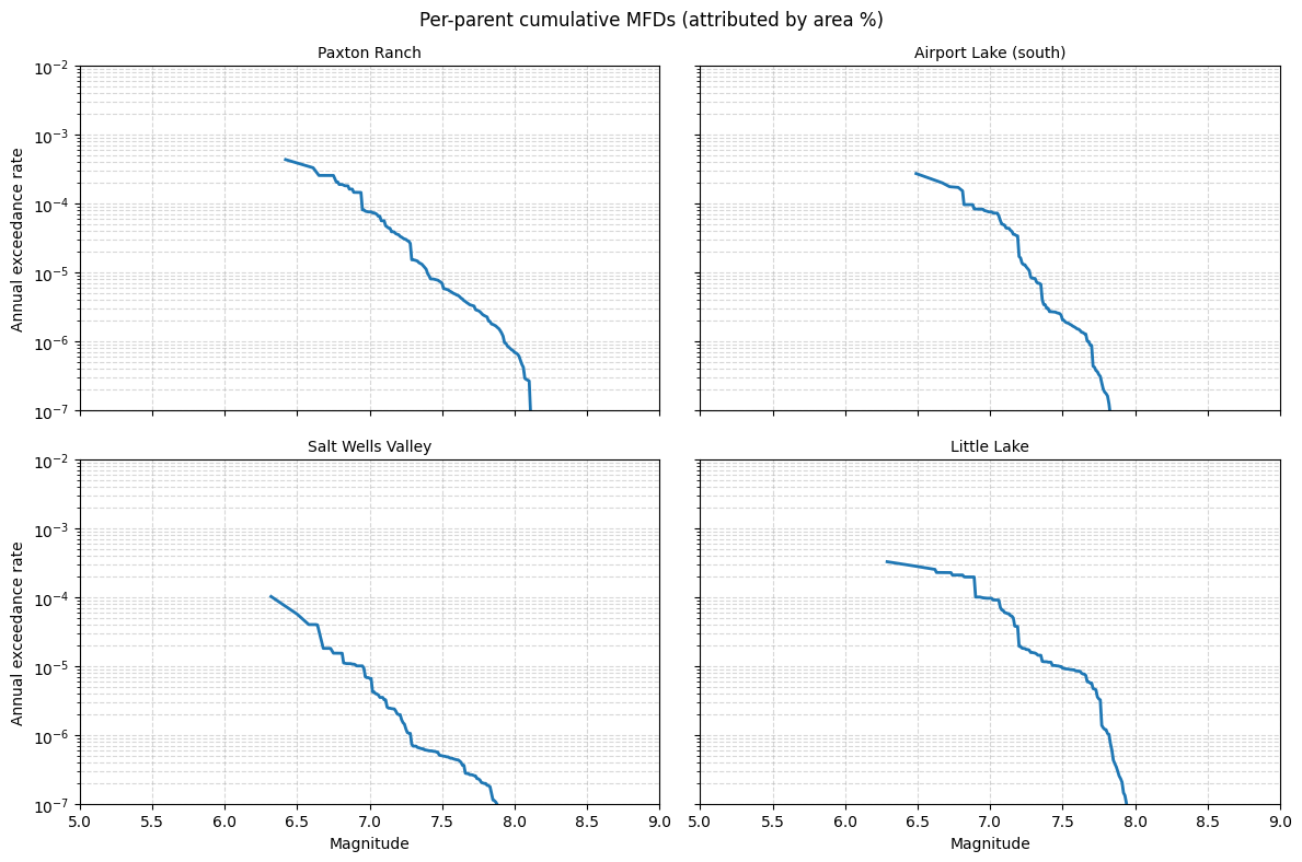
# Example: build per-parent magnitude-rate distributions.
# Explode the per-parent contributions into one row per (rupture, parent), then attribute rate.
exploded = rups.explode("contributions")
exploded[["parent_id", "area_pct"]] = pd.DataFrame(
    exploded["contributions"].tolist(), index=exploded.index
)
exploded["attributed_rate"] = exploded["rate"] * exploded["area_pct"] / 100.0

fig, axes = plt.subplots(2, 2, figsize=(12, 8), sharex=True, sharey=True)
example_pids = sel.parent_ids[:4]

for ax, pid in zip(axes.flat, example_pids):
    parent_rups = exploded[exploded["parent_id"] == pid]
    binned = parent_rups.groupby("m")["attributed_rate"].sum()
    cumulative = binned.sort_index(ascending=False).cumsum().sort_index()
    ax.semilogy(cumulative.index, cumulative.values, linewidth=2)
    ax.set_title(parents.loc[pid, "parent_name"], fontsize=10)
    ax.grid(True, which="both", linestyle="--", alpha=0.5)
    ax.set(xlim=(5, 9), ylim=(1e-7, 1e-2))

axes[1, 0].set_xlabel("Magnitude")
axes[1, 1].set_xlabel("Magnitude")
axes[0, 0].set_ylabel("Annual exceedance rate")
axes[1, 0].set_ylabel("Annual exceedance rate")

fig.suptitle("Per-parent cumulative MFDs (attributed by area %)", fontsize=12)
plt.tight_layout()
plt.show()
3. GridSelection
GridSelection filters the background gridded seismicity to points within a geodesic
distance of a site. It uses a separate radius from ParentSelection to allow the
grid extent to differ from the fault search radius.
gs = GridSelection(ds, lat=35.77, lon=-117.60, dist_km=100)
grid = gs.grid
print(f"{len(grid)} grid points within 100 km")
print("Columns:", list(grid.columns[:6]), "...")
grid[["lon", "lat", "ss_wt", "r_wt", "n_wt", "5.05", "7.85", "dist_km"]].head(10)
312 grid points within 100 km
Columns: ['lon', 'lat', 'ss_wt', 'r_wt', 'n_wt', '5.05'] ...
| lon | lat | ss_wt | r_wt | n_wt | 5.05 | 7.85 | dist_km | |
|---|---|---|---|---|---|---|---|---|
| 0 | -117.6 | 35.8 | 0.5 | 0.0 | 0.5 | 0.001287 | 3.459760e-09 | 3.328651 |
| 1 | -117.6 | 35.7 | 0.5 | 0.0 | 0.5 | 0.001007 | 5.075090e-09 | 7.766787 |
| 2 | -117.5 | 35.8 | 0.5 | 0.0 | 0.5 | 0.000303 | 9.978070e-08 | 9.634084 |
| 3 | -117.7 | 35.8 | 0.5 | 0.0 | 0.5 | 0.000987 | 5.036740e-09 | 9.634084 |
| 4 | -117.5 | 35.7 | 0.5 | 0.0 | 0.5 | 0.000451 | 2.435150e-08 | 11.923127 |
| 5 | -117.7 | 35.7 | 0.5 | 0.0 | 0.5 | 0.000577 | 4.274360e-09 | 11.923127 |
| 6 | -117.6 | 35.9 | 0.5 | 0.0 | 0.5 | 0.000243 | 7.960200e-09 | 14.424273 |
| 7 | -117.5 | 35.9 | 0.5 | 0.0 | 0.5 | 0.000153 | 6.375460e-08 | 17.020365 |
| 8 | -117.7 | 35.9 | 0.5 | 0.0 | 0.5 | 0.000334 | 4.150100e-09 | 17.020365 |
| 9 | -117.4 | 35.8 | 0.5 | 0.0 | 0.5 | 0.000155 | 5.744290e-08 | 18.385388 |